Learn hydrological modelling with airGRteaching
Olivier Delaigue
1 Hydrological modelling in three steps
This part explains how to run the airGR hydrological models in only three simple steps with airGRteaching.
1.1 Preparation of input data
A data.frame of daily hydrometeorological observations
time series at the catchment scale is needed. The required fields
are:
- DatesR: dates in the
POSIXtformat - P: average precipitation [mm/time step]
- T: catchment average air temperature [℃] [OPTIONAL]
- E: catchment average potential evapotranspiration [mm/time step]
- Qmm: outlet discharge [mm/time step]
##       DatesR    P   E    Qmm    T
## 1 1984-01-01  4.1 0.2 0.6336  0.5
## 2 1984-01-02 15.9 0.2 0.8256  0.2
## 3 1984-01-03  0.8 0.3 2.9280  0.9
## 4 1984-01-04  0.0 0.3 1.8240  0.5
## 5 1984-01-05  0.0 0.1 1.5000 -1.6
## 6 1984-01-06  0.0 0.3 1.3560  0.9
Before running a model, airGRteaching functions require data and options with specific formats.
For this step, you just have to use the PrepGR()
function. You have to define:
ObsDF:data.frameof hydrometeorological observations time seriesHydroModel: the name of the hydrological model you want to run (GR1A, GR2M, GR4J, GR5J, GR6J, GR4H or GR5H)CemaNeige: if you want or not to use the snowmelt and accumulation model
If you want to use CemaNeige, you also have to define:
- catchment average air temperature in
ObsDFor inTempMean HypsoData: a vector of 101 reals: min, quantiles (1 % to 99 %) and max of catchment elevation distribution [m]; if not defined a single elevation layer is used for CemaNeigeNLayers: the number of elevation layers requested [-]
1.2 Calibration step
To calibrate a model, you just have to use the CalGR()
function. By default, the objective function used is the Nash–Sutcliffe
criterion ("NSE"), and the warm-up period is automatically
set (depends on model). You just have to define:
PrepGR: the object returned by thePrepGR()functionCalPer: a vector of 2 dates to define the calibration period
You can obviously define another objective function or warm-up period:
CalCrit: name of the objective function ("NSE", "KGE", "KGE2", "RMSE")WupPer: a vector of 2 dates to define the warm-up period
The calibration algorithm has been developed by Claude Michel
(Calibration_Michel() function in the airGR package) .
CAL <- CalGR(PrepGR = PREP, CalCrit = "KGE2",
             WupPer = NULL, CalPer = c("1990-01-01", "1993-12-31"))
## Grid-Screening in progress (0% 20% 40% 60% 80% 100%)
## Screening completed (243 runs)
## Param = 175.915, -0.110, 83.931, 1.857, 0.467
## Crit. KGE2[Q] = 0.8300
## Steepest-descent local search in progress
## Calibration completed (18 iterations, 406 runs)
## Param = 188.670, 1.456, 83.931, 1.779, 0.493
## Crit. KGE2[Q] = 0.87871.3 Simulation step
To run a model, please use the SimGR() function. The
PrepGR and WupPer arguments of
SimGR() are similar to the ones of the CalGR()
function. Here, EffCrit is used to calculate the
performance of the model over the simulation period SimPer
and Param is the object returned by the
CalGR() function.
SIM <- SimGR(PrepGR = PREP, Param = CAL, EffCrit = "KGE2",
             WupPer = NULL, SimPer = c("1994-01-01", "1998-12-31"))
## Crit. KGE2[Q] = 0.8549## SubCrit. KGE2[Q] cor(sim, obs, "pearson") = 0.9012
## SubCrit. KGE2[Q] cv(sim)/cv(obs) = 0.8974
## SubCrit. KGE2[Q] mean(sim)/mean(obs) = 0.97242 Formating outputs
The call of the as.data.frame() function with
PrepGR, CalGR or SimGR objects
allows to coerce the outputs to a data frame.
##        Dates PotEvap PrecipObs PrecipFracSolid_CemaNeige TempMeanSim_CemaNeige   Qobs Qsim
## 1 1984-01-01     0.2       4.1                        NA                    NA 0.6336   NA
## 2 1984-01-02     0.2      15.9                        NA                    NA 0.8256   NA
## 3 1984-01-03     0.3       0.8                        NA                    NA 2.9280   NA
## 4 1984-01-04     0.3       0.0                        NA                    NA 1.8240   NA
## 5 1984-01-05     0.1       0.0                        NA                    NA 1.5000   NA
## 6 1984-01-06 0.3 0.0 NA NA 1.3560 NA## Dates PotEvap PrecipObs PrecipFracSolid_CemaNeige TempMeanSim_CemaNeige Qobs Qsim
## 1 1990-01-01 0.3 0.0 NA NA 1.992 2.523954
## 2 1990-01-02 0.4 9.3 NA NA 1.800 2.446199
## 3 1990-01-03 0.4 3.2 NA NA 2.856 2.943436
## 4 1990-01-04 0.3 7.3 NA NA 2.400 3.286214
## 5 1990-01-05 0.1 0.0 NA NA 3.312 3.512572
## 6 1990-01-06 0.1 0.0 NA NA 3.072 3.224969## Dates PotEvap PrecipObs PrecipFracSolid_CemaNeige TempMeanSim_CemaNeige Qobs Qsim
## 1 1994-01-01 0.4 2.2 NA NA 2.904 3.593023
## 2 1994-01-02 0.4 0.0 NA NA 2.832 3.414026
## 3 1994-01-03 0.6 0.7 NA NA 2.364 2.988078
## 4 1994-01-04 0.6 3.2 NA NA 2.544 2.668972
## 5 1994-01-05 0.6 35.1 NA NA 2.640 3.526016
## 6 1994-01-06 0.5 21.3 NA NA 8.928 8.8199353 Pre-defined graphical plots
3.1 Static plots
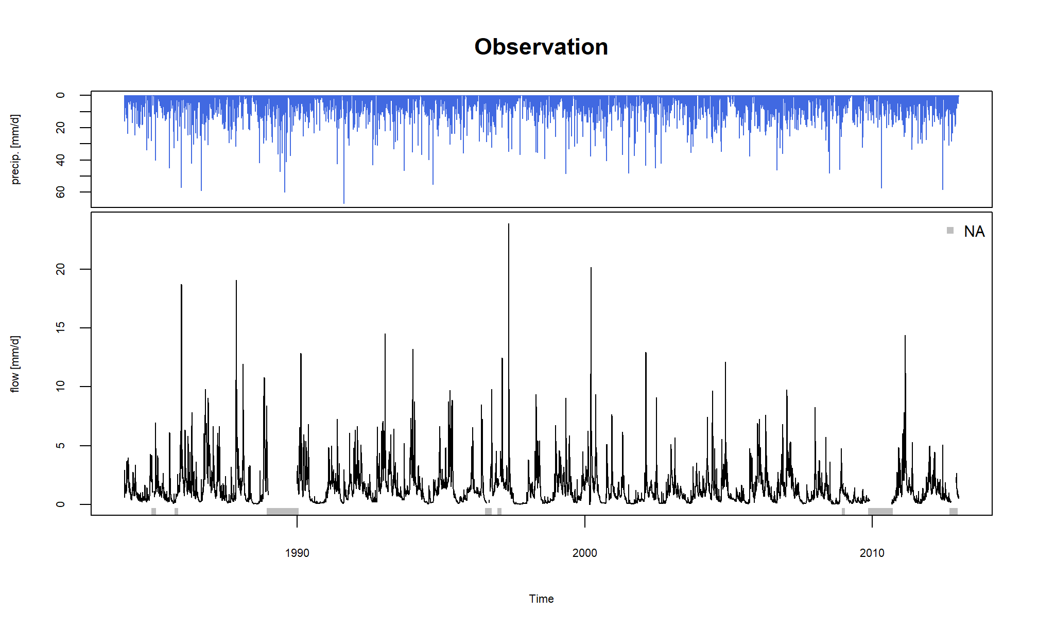
The call of the plot() function with a
PrepGR object draws the observed precipitation and
discharge time series.
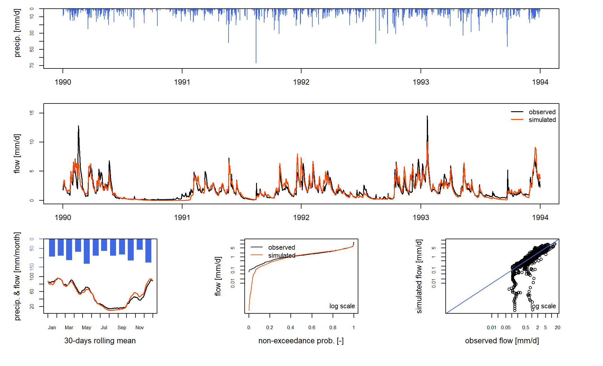
By default (with the argument which = "synth"), the call
of the plot() function with a CalGR object
draws the classical airGR
plot diagnostics (observed and simulated time series together with
diagnostic plot)
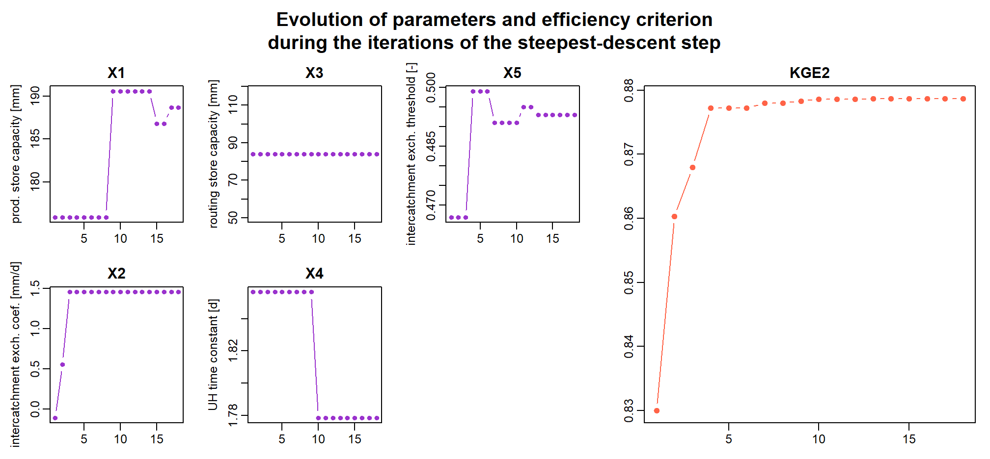
With the CalGR object, if the argument
which is set to "iter", the
plot() function draws the evolution of the parameters and
the values of the objective function during the second step of the
calibration (steepest descent local search algorithm):
With the CalGR object, if the argument
which is set to "ts", the plot()
function simply draws the time series of the observed precipitation, and
the observed and simulated flows:
## Warning in plot.OutputsModel(x$OutputsModel, Qobs = x$Qobs, which = which, : zeroes detected in 'Qsim': some
## plots in the log space will not be created using all time-steps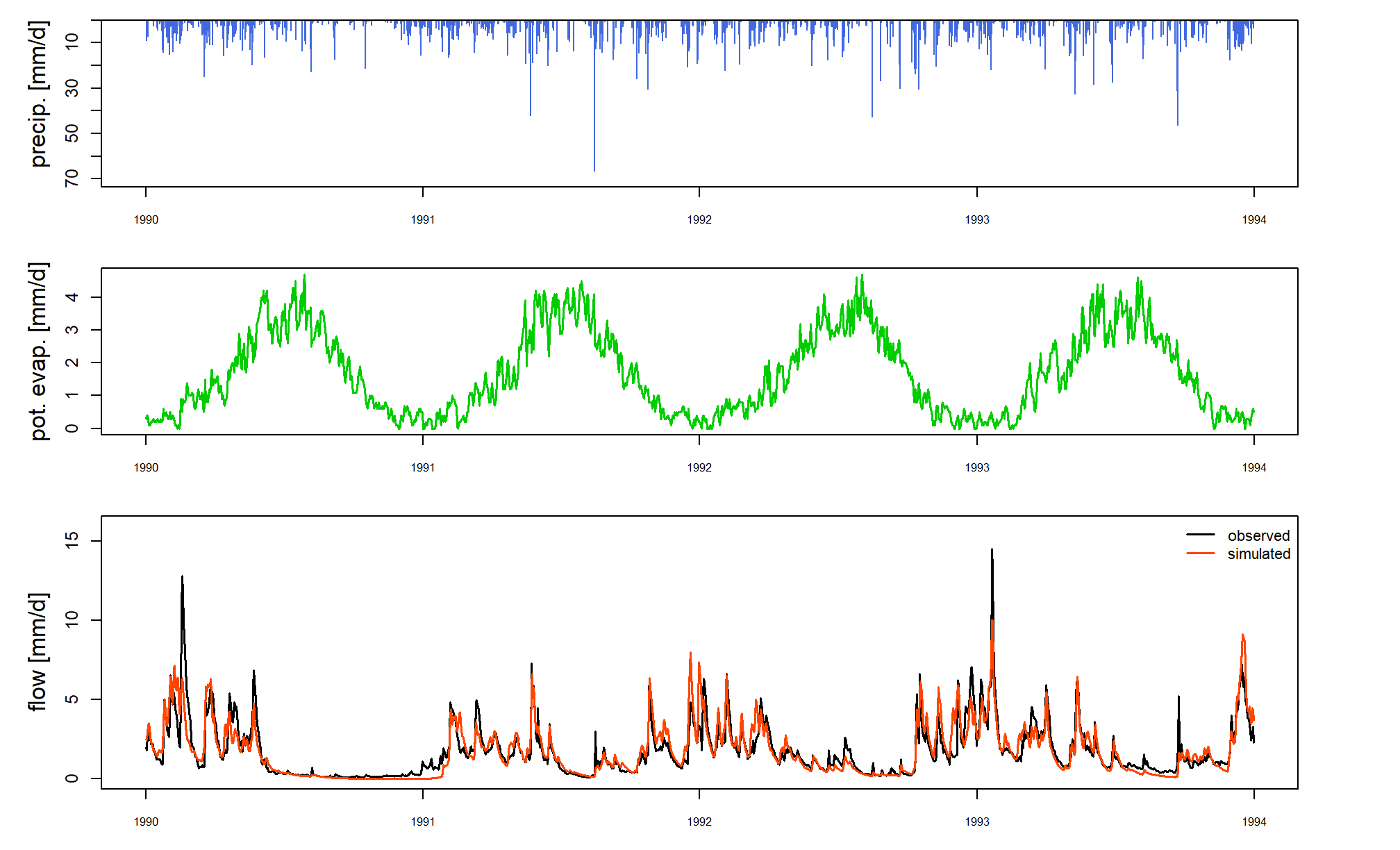
The call of the plot() function with a
SimGR object displays the classical airGR plot diagnostics.
3.2 Dynamic plots
Dynamic plots, using the dygraphs JavaScript charting library, can be displayed by the package.
The dyplot() function can be applied on
PrepGR, CalGR and SimGR objects
and draws the time series of the observed precipitation, and the
observed and simulated (except with PrepGR objects)
flows.
The user can zoom on the plot device and can read the exact values.
With this function, users can easily explore the data time series and also explore and interpret the possible problems of the calibration or simulation steps.
4 Graphical user interface
The airGRteaching
package also provides the ShinyGR() function, which allows
to launch a graphical user interface using the shiny
package.
The ShinyGR() function needs at least:
ObsDF: a (list of)data.frame(or independant vector instead, see?ShinyGR)SimPer: a (list of) vector(s) of 2 dates to define the simulation period(s)
Only the monthly model (GR2M) and the daily models (GR4J, GR5J, GR6J
+ CemaNeige) are currently available.
If you want to use CemaNeige, you also have to define the same arguments
desribed above for the PrepGR() function.
It is also possible to change the interface look; different themes
are proposed (theme argument).